LDA Autotagging process 를 알아봅시다.
본 프로젝트의 목적은 정보과 과부화되고, 정리되지 않은 관보 문서들에게, 그들이 가지고 있는 주제와 산업군을 바탕으로 검색의 용이성을 만드는데 목적이 있습니다. 본 과정을 어떻게 진행하면 좋을지 이야기해 봅시다.
사용한 라이브러리는 다음과 같습니다.
1
2
3
4
5
6
7
8
9
10
11
12
13
import os
import json, requests
from pymongo import MongoClient
import pandas as pd
import numpy as np
import matplotlib.pyplot as plt
import re
import coredottext.nlp as nlp
import pyLDAvis.gensim
from gensim import corpora
from gensim.corpora import Dictionary
from gensim.models.ldamodel import LdaModel
%pylab inline
Data를 넣어봅시다
지난번에 전처리하고 파라미터를 튜닝했었던 문서를 다시 호출해 봅시다.
1
2
3
4
5
6
7
8
from gensim import corpora, models, similarities
import os
if (os.path.exists('stop&bi(min=2,threshold=50,no_above=0.5).dict')):
    dictionary = corpora.Dictionary.load('stop&bi(min=2,threshold=50,no_above=0.5).dict')
    corpus = corpora.MmCorpus('stop&bi(min=2,threshold=50,no_above=0.5).mm')
    print("Dictionary와 corpus가 준비되었습니다!")
else:
    print("데이터가 없어요!")
Process 정리
위 아이디어를 구현하기 위해서 우리가 알아야 하는것은, doc_topic_dist, doc_corpus, topic_term_dist 이렇게 3가지입니다. 하지만 corpus, dictionary, LDA 모형에서 이미 우리는 알고 있습니다. 토픽의 관점, 문서의 관점, 그리고 단어의 관점을 살펴보면서 해당 개념들을 익혔습니다.
1
2
print("unique token: %d" % len(dictionary))
print("number of documents: %d" % len(corpus))
1. Doc_term matrix : Bow에서 Sparse Matrix 로
저희가 살펴볼 첫번째 개념은 Doc_term matrix입니다. 우리가 만들어낼 doc_topic, topic_term과 같은 분포에 원 재료가 되어주는 matrix입니다. 문서는 단어로 구성되어 있고, 단어는 LDA의 최소단위라고 생각하시면 됩니다.
gensim.matutils.corpus2csc(corpus, num_terms=None, dtype=<type ‘numpy.float64’>, num_docs=None, num_nnz=None, printprogress=0)
Bag of Word 포맷을 scipy.sparse.csc_matrix 로 바꾸게 됩니다. column이 documents 이고 row가 term인 matrix로 반환된다.
Parameters:
- corpus (iterable of iterable of (int, number)) – BoW format의 말뭉치를 넣어줍시다.
- num_terms (int, optional) – 말뭉치에 있는 term의 갯수입니다. dictionary의 길이를 넣어줍시다.
- dtype (data-type, optional) – output CSC matrix 의 데이터 타입을 지정할 수 있습니다. 디폴트는 numpy.float 64값을 받습니다.
- num_docs (int, optional) – 말뭉치에 들어간 documents의 갯수를 조절 가능합니다.
- num_nnz (int, optional) – 말뭉치에 non-zero elements 를 지정할 수 있습니다.
- printprogress (int, optional) – Log a progress message at INFO level
1
2
3
4
#Sparse matrix로 변환시켜 봅시다.
corpus_csc = gensim.matutils.corpus2csc(corpus, num_terms=len(dictionary))
corpus = gensim.matutils.Sparse2Corpus(corpus_csc)
corpus_csc
<1289x202 sparse matrix of type '<class 'numpy.float64'>'
	with 16179 stored elements in Compressed Sparse Column format>
1289개의 토큰이 202개의 문서에 numpy.float64의 형태로 저장되어 있군요!
2. Term-frequency matrix를 만들어 봅시다.
각 단어별 문서에 등장한 frequency가 두번째 재료가 되어줍니다.
1
2
3
4
5
6
7
8
9
10
11
12
13
14
15
16
17
# dictionary에서 단어를 뽑아내 봅시다.
vocab = list(dictionary.token2id.keys())
beta = 0.01

# 토큰 id로 array를 만든 것이다. 왜냐면 topic term matrix를 만들어야 하거든요!
fnames_argsort = np.asarray(list(dictionary.token2id.values()), dtype=np.int_)
# term frequency distribution을 만든 것이다.
term_freqs = corpus_csc.sum(axis=1).A.ravel()[fnames_argsort]

# term_freqs가 0인 친구들에게 beta 값을 넣는다
term_freqs[term_freqs == 0] = beta

# 문서의 길이를 token을 바탕으로 계산한다
doc_lengths = corpus_csc.sum(axis=0).A.ravel()\

# 토픽 갯수를 저장
num_topics = LDA.num_topics
3. Documents-Topic Distribution 을 만들어 봅시다.
Document에 어떤 topic이 지배적으로 등장하는지에 대한 확률값은 LDA의 infernece함수를 통해서 찾아낼 수 있습니다.
inference(chunk, collect_sstats=False)
만약 sparse document vector가 존재한다면, 각각 문서에 대하여 topic weights의 감마값을 추정해줍니다.
Avoids computing the phi variational parameter directly using the optimization presented in Lee, Seung: Algorithms for non-negative matrix factorization”.
Parameters:
chunk ({list of list of (int, float), scipy.sparse.csc}) – 말뭉치를 넣어주면 됩니다. collect_sstats (bool, optional) – 만약 True로 둔다면, 모형의 doc-term distributions의 sufficient statistics를 리턴한다고 하네요!
Returns:
- gamma matrix 추정 값을 리턴하며
- collect sstats를 Ture로 놓을 시 EM 알고리즘 중 E step의 sufficient statistics을 리턴합니다.
1
2
3
4
# LDA inference 함수를 통해
gamma, _ = LDA.inference(corpus)
doc_topic_dists = gamma / gamma.sum(axis=1)[:, None]
doc_topic_dists
array([[1.9330212e-01, 4.6853849e-05, 3.5728863e-05, ..., 3.1558979e-05,
        3.4545526e-05, 2.7846638e-05],
       [3.7254574e-04, 4.9023226e-01, 3.9519093e-04, ..., 3.4906855e-04,
        3.8210227e-04, 3.0800697e-04],
       [5.2947836e-04, 1.3118789e-01, 5.6166272e-04, ..., 4.9611158e-04,
        5.4306054e-04, 8.1526726e-02],
       ...,
       [5.8416167e-04, 8.1261818e-04, 6.1966997e-04, ..., 5.4734881e-04,
        5.9914659e-04, 4.8296319e-04],
       [6.5144087e-04, 8.4783949e-02, 6.9103873e-04, ..., 6.1038823e-04,
        4.8515934e-01, 5.3858710e-04],
       [5.9964403e-04, 8.3415542e-04, 6.3609338e-04, ..., 5.6185550e-04,
        6.1502605e-04, 4.9576344e-04]], dtype=float32)
4. Topic-Term Distribution 을 만들어 봅시다.
LDA.state.get_lambda()
각 term에 부여되어 있는 topic의 posterior 확률을 받아볼 수 있습니다.
1
2
3
topic = LDA.state.get_lambda()
print(topic.shape)
topic
(30, 1289)
array([[0.04614676, 0.31315815, 0.06789937, ..., 0.02703826, 0.03091238,
        0.02703826],
       [0.04614676, 2.1075764 , 0.06789931, ..., 0.02703826, 0.03091238,
        0.02703826],
       [0.04614676, 3.5415056 , 0.06789931, ..., 0.02703826, 0.03091238,
        0.02703826],
       ...,
       [0.04614676, 0.30416465, 0.06830934, ..., 0.02703826, 0.03091238,
        0.02703826],
       [0.04614676, 0.291997  , 0.06789931, ..., 0.02703826, 0.03091238,
        0.02703826],
       [0.04614676, 0.29362017, 1.0627426 , ..., 0.02703826, 0.03091238,
        0.02703826]], dtype=float32)
1
2
3
topic = topic / topic.sum(axis=1)[:, None]
topic_term_dists = topic[:, fnames_argsort]
topic_term_dists
array([[1.97014342e-05, 1.33696609e-04, 2.89882755e-05, ...,
        1.15434450e-05, 1.31974193e-05, 1.15434450e-05],
       [3.47235109e-05, 1.58586330e-03, 5.10913997e-05, ...,
        2.03451655e-05, 2.32602724e-05, 2.03451655e-05],
       [6.87927386e-05, 5.27945766e-03, 1.01220096e-04, ...,
        4.03069716e-05, 4.60822594e-05, 4.03069716e-05],
       ...,
       [3.37744605e-05, 2.22615796e-04, 4.99950911e-05, ...,
        1.97891004e-05, 2.26245320e-05, 1.97891004e-05],
       [1.03068400e-04, 6.52172836e-04, 1.51652537e-04, ...,
        6.03897352e-05, 6.90425295e-05, 6.03897352e-05],
       [1.80663963e-04, 1.14951911e-03, 4.16062353e-03, ...,
        1.05854444e-04, 1.21021541e-04, 1.05854444e-04]], dtype=float32)
1
2
input_dict = {'topic_term_dists': topic_term_dists, 'doc_topic_dists': doc_topic_dists,
            'doc_lengths': doc_lengths, 'vocab': vocab, 'term_frequency': term_freqs}
완성되었습니다. 원래 필요했던 소스들이 모두 완성되었습니다.
쉽게 구현해보는 코드!
Gensim에서는 이미 구현되어 있습니다!
1
2
3
4
5
6
7
8
9
10
11
12
13
14
15
16
17
18
19
20
21
22
23
24
25
26
27
28
29
30
31
32
33
34
35
36
37
38
39
40
def making_input(model, all_corpus, doc_dictionary):
    extract = pyLDAvis.gensim._extract_data(model, all_corpus, doc_dictionary)
    topic_term_dists = extract['topic_term_dists']
    doc_topic_dists = extract['doc_topic_dists']
    doc_lengths = extract['doc_lengths']
    vocab = extract['vocab']
    term_frequency = extract['term_frequency']
    topic_term_dists = pyLDAvis._prepare._df_with_names(topic_term_dists, 'topic', 'term')
    doc_topic_dists  = pyLDAvis._prepare._df_with_names(doc_topic_dists, 'doc', 'topic')
    term_frequency   = pyLDAvis._prepare._series_with_name(term_frequency, 'term_frequency')
    doc_lengths      = pyLDAvis._prepare._series_with_name(doc_lengths, 'doc_length')
    vocab            = pyLDAvis._prepare._series_with_name(vocab, 'vocab')
    pyLDAvis._prepare._input_validate(topic_term_dists, doc_topic_dists, doc_lengths, vocab, term_frequency)

    topic_freq       = (doc_topic_dists.T * doc_lengths).T.sum()
    # topic_freq       = np.dot(doc_topic_dists.T, doc_lengths)
    if (True):
        topic_proportion = (topic_freq / topic_freq.sum()).sort_values(ascending=False)
    else:
        topic_proportion = (topic_freq / topic_freq.sum())

    topic_order      = topic_proportion.index
    # reorder all data based on new ordering of topics
    topic_freq       = topic_freq[topic_order]
    topic_term_dists = topic_term_dists.iloc[topic_order]
    doc_topic_dists  = doc_topic_dists[topic_order]

    # token counts for each term-topic combination (widths of red bars)
    term_topic_freq = (topic_term_dists.T * topic_freq).T
    ## Quick fix for red bar width bug.  We calculate the
    ## term frequencies internally, using the topic term distributions and the
    ## topic frequencies, rather than using the user-supplied term frequencies.
    ## For a detailed discussion, see: https://github.com/cpsievert/LDAvis/pull/41
    term_frequency = np.sum(term_topic_freq, axis=0)

    topic_info         = pyLDAvis._prepare._topic_info(topic_term_dists, topic_proportion, term_frequency, term_topic_freq, vocab, 0.01, 50, -1)
    token_table        = pyLDAvis._prepare._token_table(topic_info, term_topic_freq, vocab, term_frequency)
    client_topic_order = [x + 1 for x in topic_order]

    return topic_info
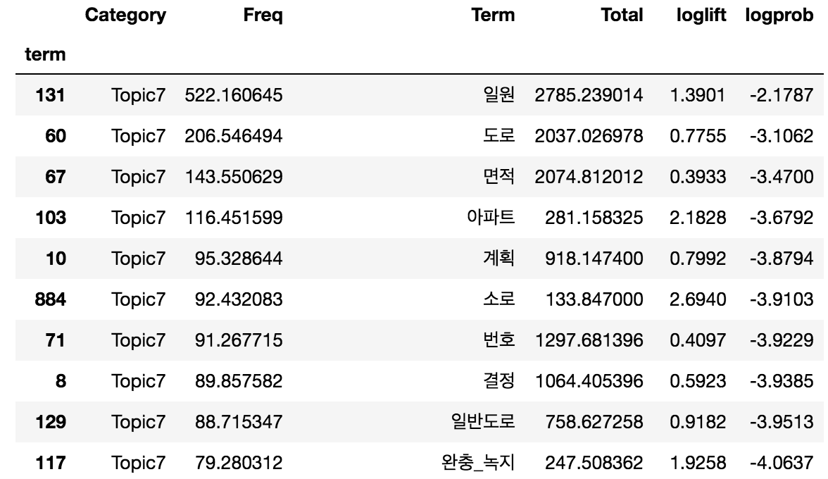
한번 도로라는 term이 속해있던 Topic7번을 조회해 볼까요?, 저는 pyLDAvis에서 lamdba값을 0으로 만들었을때 중요했던 logprob를 기준으로 정렬시켜보겠습니다.
1
df_input[df_input.Category == 'Topic7'].sort_values(by=['logprob'], ascending = False)
sorting 이 완료된 후 인덱스를 받아오고 싶다면
1
df_input[df_input.Category == 'Topic7'].sort_values(by=['logprob'], ascending=False).index
Int64Index([ 131,   60,   67,  103,   10,  884,   71,    8,  129,  117,   72,
             813,   52, 1044,  560,  163, 1037,   95,  152,  120,  158,  668,
             870,  249,   81,  336,    5,  346, 1011,  781,   27,   33,   76,
            1069,  126,  147, 1087,  794,  663, 1278,   47,  218, 1079,   73,
            1203, 1007,  327,   97,   23,  675,   39, 1238,  465,  680,   66,
             144,  151,   90,  816,  329,  783,  682, 1221,  804,  894,  685,
            1240, 1033, 1241,  866, 1064, 1154,  168, 1030,  109,  803,  566,
             167, 1036,  136,  407, 1235,    2, 1024,  844,  110,  909,  801,
            1081,  795,  802,  968, 1186, 1274, 1123,  581, 1272],
           dtype='int64', name='term')
이제 tagging process로 넘어가보자!
1
2
3
4
5
6
7
8
9
10
11
12
13
14
15
16
17
18
19
20
21
22
23
24
25
26
27
def Keyword_tagging(model, all_corpus ,doc_corpus, doc_dictionary):
    # doc 코퍼스에서 가장 높은 확률의 topic 3개를 뽑는다. 그후 정렬한다.
    doc_topic_dist = model.get_document_topics(doc_corpus, minimum_probability=0.3)
    sorted_doc_topic = sorted(doc_topic_dist, key=lambda x:x[1], reverse=True)

    # 람다의 변화에 맞는 term을 받기 위해, input dataframe 을 만든다
    df_input = making_input(model, all_corpus, doc_dictionary)

    # 각 토픽을 대표하는 topic-term list를 받는다.
    tagging_word = []
    for i, j in sorted_doc_topic:
        # 토픽을 대표하는 텀의 갯수
        topic_term_list_id = df_input[df_input.Category == 'Topic'+str(i)].sort_values(by=['logprob']).index
        # doc_corpus 값 역시, word-id, frequency로 분해한다.
        doc_corpus_id, doc_corpus_frequency = zip(*doc_corpus)
        topic_term_list_id = list(topic_term_list_id)
        doc_corpus_id = list(doc_corpus_id)

        # topic_term_list_id 와 doc_corpus_id를 비교하여 공통되는 친구들을 return 한다.
        target = []
        for a in doc_corpus_id:
            if a in topic_term_list_id:
                target.append(a)
                words = [doc_dictionary[word_id] for word_id in target]
                tagging_word.extend(words)

    return(set(tagging_word))
1
Keyword_tagging(LDA,corpus,corpus[1],dictionary)
{'도로', '번호', '성명', '제조', '주소', '추가'}
지난 post에서 corpus[1]은 도로 topic과 관련이 높은 term이 들어간 documents였습니다. 다시확인해볼까요
1
2
words = [dictionary[word_id] for word_id, count in corpus[1]]
print(words)
['도로', '번호', '유치원', '주소', '경과', '국민_행정절차법', '기관단체_단체명', '기관단체_통합', '대표_자명', '도로법', '도움', '마련', '명시', '민간', '반대_이유', '부개_정령', '부칙', '사항_기재', '사항_우편', '성명', '세종_특별자치시', '예고_사항', '예방', '을 ', '의견서_국토교통부장관', '의견제출_개정안', '이유_주요', '입법예고', '입법예고_이유', '전자우편_팩스', '제한', '조항', '주요', '찬성_반대', '참고', '추가', '출입', '국토교통부장관', '제조']
나쁘지않게 토픽이 tagging된것으로 보입니다.